Graph Database Fundamentals
Graph databases are on the rise, but amid all the hype it can be hard to understand graph database differences under the hood. This blog is not marketing or a tutorial — it’s an attempt to give a clear description of strengths and weaknesses.
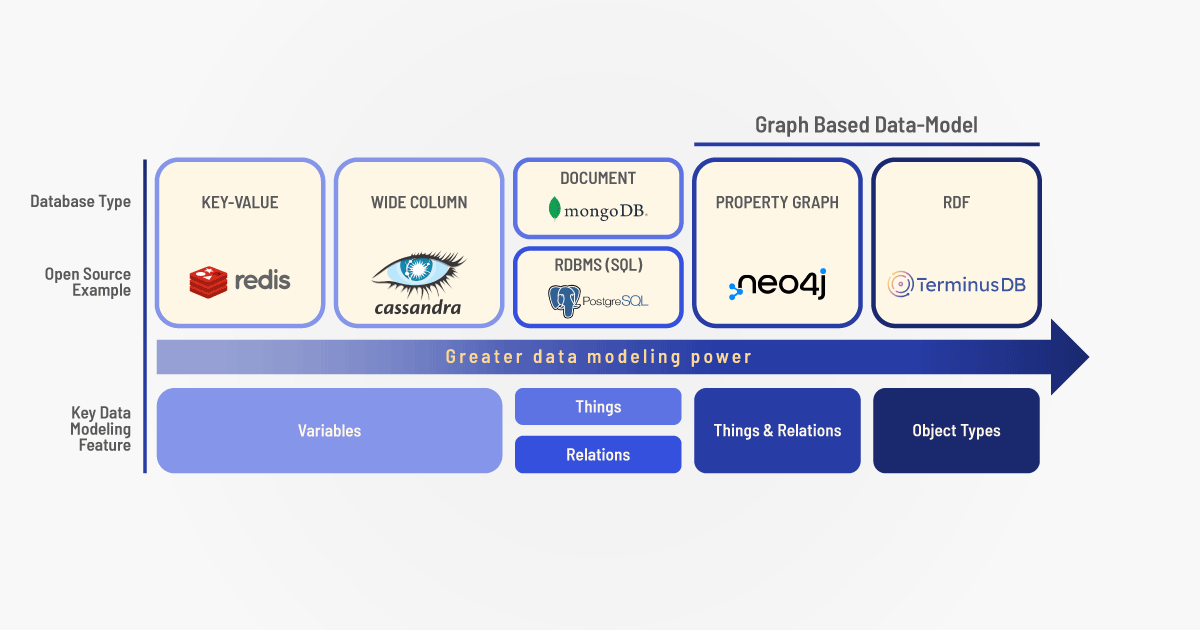
There are two major variants of graph database in the wild — RDF graphs (aka triple-stores) and Labeled Property Graphs.
RDF – Resource Description Framework
RDF is a child of the web, formulated back in the 1990s, by Tim Bray at Netscape as a meta-data schema for describing things. The basic idea is simple, RDF files consist of a set of logical assertions: subject, predicate, object — known as a triple:
subject -> predicate -> object
Each triple expresses a specific fact about a subject:
					    mary -> likes -> john
    mary -> is    -> human
    john -> likes -> jane
    jane -> likes -> chocolate
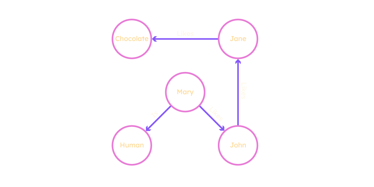
When joined together a set of triples forms a graph consisting of nodes and edges — it really is as simple as that.
Triples can be combined to represent a knowledge graph that computers can interpret and reason about. When joined together, they form a natural graph, where the predicates (the middle part of the triple) are interpreted as edges and the subjects and objects are the nodes.
So far so good. In fact, triples are an excellent atom of information — 3 degrees of freedom in our basic atomic expressions is sufficient for a self-describing system. We can build up a set of triples that describes anything describable. Binary relations, on the other hand, which are the basis of tables and traditional databases, can never be self-describing: they will always need some logic external to the system to interpret them — 2 degrees of freedom is insufficient.
The triple as a logical assertion is also a tremendously good idea — one consequence is that we don’t have to care about duplicate triples — if we tell the computer that Mary likes John a million times, it is the same as telling it once — a true fact is no more nor less true if we say it 1000 times or once.
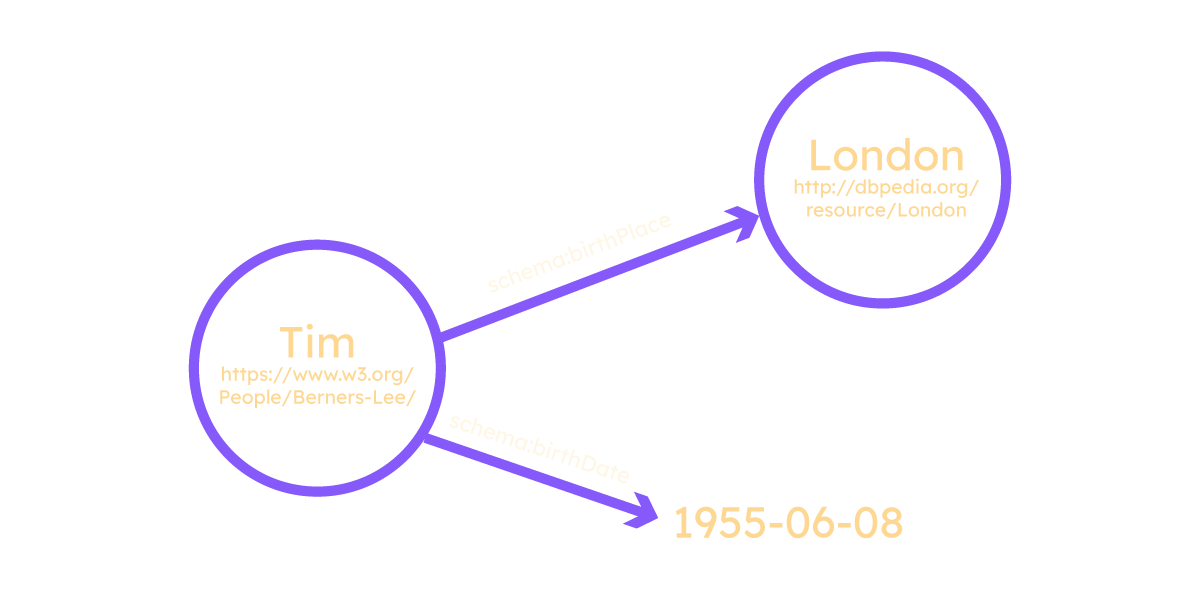
But RDF defined a lot more than just the basic idea of subject-predicate-object logical assertion triples. It also defined a naming convention where both the subject and predicate of each triple had to be expressed as a URI (often referred to as Uniform Resource Locators, URLs). The object of each triple could either be expressed as a URI or as a literal, such as a number “6”, or string “hat”. Using the above graph database example, our triples need to be in the form:
http://my.uri/john -> http://my.uri/likes -> http://my.uri/jane
The basic idea is that if we load the URI of any subject, predicate, or object, we will find the definition of the node or edge in question at that URI. So, if we load http://my.uri/likes into our browser, we find the definition of the likes predicate. This design decision has both costs and benefits.
The cost is immediate — URIs are much longer than the variable names used in programming language and they are hard to remember. This slows down programming as we can’t just use simple strings as usual, we have to refer to things by their full URI. RDF tried to mitigate this cost by introducing the idea of namespace prefixes. That is to say, we can define: prefix ex = http://my.uri/ and then we can refer to john as ex:john rather than the full URI http://my.uri/john.
From a programming point of view, these namespace prefixes certainly make it much easier to use RDF, but there is still considerable cost over traditional simple variable names — we have to remember which prefixes are available, which entities and predicates belong to which namespace, and type several extra characters for every variable.
In programming, productivity is dependent on reducing the number of things that we have to remember at each step because we are concentrating on a big picture problem and need to focus all our concentration there rather than on the details of the lines of code. From that point of view, using URIs as variable names, even with prefixes, is a cost to programming speed.
The benefits, on the other hand, are seen in the medium and long term. There is an old computer science joke:
There are only 2 hard things in computer science: naming things, cache coherence, and off-by-one errors.
This is a good joke because it is true — naming things and cache coherence really are the hardest things to get right — while off-by-one errors are just extremely common errors that novices make in loop control.
RDF helps significantly to address both of the hard problems — by forcing coders to think about how they name things and by using an identifier that is uniformly and universally addressable, the problem of namespace clashes (people using the same name to talk about different things) is greatly reduced. What’s more, linking an entity to its definition greatly helps the cache coherence problem — everything has an authoritative address at which the latest definition is available.
From an overall systems perspective, the extra pain is potentially worth it — if we know how something is named, we can always look it up and see what it is. By contrast, when we are dealing with relational databases, the names used have no meaning outside the context of the local database — tables, rows, and columns all have simple variable names which mean nothing except within the particular database in which they live, and there is no way of looking up the meaning of these tables and columns because it is opaque — embedded in external program code.
RDF, however, is much more than just the basic triple form. It also defines a set of reusable predicates. The most important one of these is rdf:type — this allows the definition of entities as having a particular type:
ex:mary -> rdf:type -> ex:human
This triple example defines mary as being of type ‘human’. This provides us with the basis for constructing a formal logic in which we can reason about the properties of things based on their types — if we know mary is a human and not, for example, a rock, we can probably infer things about her without knowing them directly.
Formal logics are very powerful because they can be interpreted by computers to provide us with a number of useful services — logical consistency, constraint checking, theorem proving, and so on. And they help tremendously in the battle against complexity — the computer can tell us when we are wrong.
The Problem With RDF
There are of course trade-offs and design decisions that aren’t so good.
RDF supports ‘blank nodes’ – nodes that are not identified by a URI but instead by a local identifier (given a pseudo prefix like “_:name”). This is supposed to represent the situation where we want to say “some entity whose name I do not know” — to capture for example assertions such as “there is a man in the car”. As we don’t know the identity of the man, we use a blank node rather than a URI to represent him.
It confuses the identity of the real-world thing with the identity of the data structure that represents it. It introduces an element into the data structure that is not universally addressable and thus cannot be linked to outside its definition for no good reason. Just because we don’t know the identity of the thing, does not and should not mean we cannot address the structure describing the unknown thing. RDF tools often interpret blank nodes in such a way that their identifiers can be changed at will, meaning that it is hard to mitigate the problem in practice. (In TerminusDB we skolemize all blank nodes).
Another potential design flaw relates to the semantics that were published to govern the interpretation of triples and their types. It is a long and technical story, but basically RDF included explicit support for making statements about statements — what is called higher order statements — without putting in place rules that prevented the construction of inconsistent knowledge bases.
Another issue is the serialization format that was chosen to express RDF textually: RDF/XML. Back in 1999, XML was relatively new and fashionable, so it was a natural choice, but the way in which RDF had to be shoehorned into XML created a sometimes confusing monster.
Back in 1999 when the RDF and RDF/XML standards were published, the social web was just taking off and a simple technology called RSS (really simple syndication) was at its core. RSS 0.91 was a very simple and popular meta-data format that allowed bloggers to easily share their updates with third-party sites, enabling people to see when their favorite site had published updates so that they didn’t have to check manually.
One of the easy-to-see-in-hindsight mistakes was pushing RDF/XML as the new standard for RSS — RSS 1.0. There was a very quick revolution of bloggers who found the new standard vastly increased the complexity of sharing updates, without giving anything extra in return. Bloggers generally stuck to the old non-RDF 0.91 version — the ideological wars that this created soured web developers on RDF (the ‘it is too complicated’ meme persists today).
There Is Hope
At its core, RDF remains one of the most advanced and sophisticated mechanisms available for describing things in a computer-interpretable way. And the standard did not remain static — the W3C issued a series of new standards that refined and extended the original RDF and built several other standards on top of it.
Labeled Property Graphs
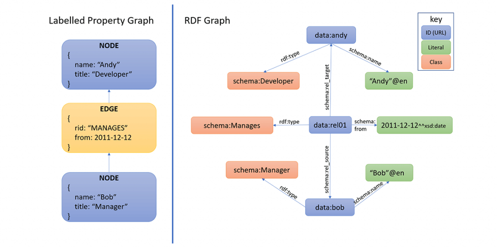
The second major graph database variant is known as a property graph or labeled property graph (LPG). Property graphs are much simpler than RDF — they consist of a set of nodes and a set of edges, with each node and edge being essentially a ‘struct’ — a simple data structure consisting of keys and values (which in some cases may themselves be structs). Nowadays JSON is the standard way of encoding these structs — each node and edge is a JSON document, with edges having special keys which indicate that the value represents a pointer to a node.
Whereas RDF uses URIs as identifiers for properties and entities, property graphs use simple strings — purely local identifiers. And while RDF uses the triple as the atom of data, property graphs do not — they are simply collections of arbitrary data structures, some of which can point at other structures. A third major difference is that RDF is intimately associated with the semantic web. There are many layers that have been built on top to provide descriptions of the semantics of the entities described in RDF graphs. Property graphs, on the other hand, do not attempt to be self-describing at all; the meaning and interpretation of the structures are left up to the consumer of the data. They are just keys and values and, with the exception of edge links and a few other special keys, you can interpret them however you want.
					CREATE (a { name: 'Andy', title: 'Developer' })
CREATE (b { name: 'Bob', title: 'Manager' })MATCH (a),(b)
WHERE a.name = 'Andy' AND b.name = 'Bob'
CREATE (b)-[r:MANAGES]->(a)
A graph db example of creating two nodes and an edge in Cypher, Neo4J’s self-rolled graph query and definition language. In the absence of universal identifiers, the nodes that were created have to be matched by a property value before the edge can be created.
To somebody coming from a semantic web background, property graphs can seem like an impoverished alternative. That said, Neo4j and its modern imitators are by far the most popular type of graph database in the world and there are some very good reasons for this.
Neo4j started out as a library for the Java programming language (hence the 4j) that enabled them to create and store graph-like data structures. The property graph people, to their credit, took a pragmatic approach and focused on making a database that ordinary humans could understand. Property graphs were always focused on the graph as the best abstraction for modeling the world. And as important use-cases emerged that used graph algorithms (fraud detection, page-rank, recommender systems) they were much better positioned to take advantage. Nodes represent things that are close to things in the world, edges represent relationships between things — all very intuitive.
One consequence of this difference is that, when it comes to property graphs, it is relatively straightforward to add meta-data to edges — they are just structs after all and you can add whatever you like to the JSON blob representing an edge. This provides a straightforward way of adding qualifiers to edges — representing time, space, or any other qualifier you want — to represent relationships with weights and lifespans, for example.
Property graphs provide a relatively simple mechanism that is easily understood by coders for modeling real-world things and qualified relationships between them. Over time, Neo4j developed, in an evolutionary way, a query language called Cypher that is reasonably intuitive for coders — including some cute ways of representing graph edges:
(a)-[relationship]->(b)
However, when dealing with very large graph dbs — billions of nodes and edges have become the norm today— their early pragmatism comes back to bite them with a vengeance. When graphs get really big and complicated, without a formal mathematical-logical basis for reasoning about graph traversals, leaving it all up to the individual query writer can be challenging as the heat death of the universe lies around every corner.
As graph databases move from being toys for enthusiastic coders into serious enterprise tools, constraints and schemata become important. The cost of early pragmatism is problematic as it is difficult to engineer such fundamental logic back into the core of the system. As systems become bigger and more interconnected, jettisoning URIs in favor of local identifiers is a serious impediment. The cost of stitching together systems of local identifiers in every new case adds up to more significant trouble than it would have been adopting URIs as universal identifiers initially.
Graph Schema Languages
Graph database schema languages attempt to support the definition of schemata — rules defining the shape of the graph. Almost all of this work has been confined to the world of RDF. Property graphs, by contrast, with their pragmatic focus on simplicity, took the approach of delegating the schema to code rather than imposing it in the data layer, only supporting low-level constraints on the basic node-edge structure.
A somewhat bewildering series of standards and extensions have been built on top of RDF, mostly standardized by the W3C standards committee. Shortly after publishing the RDF standard, the focus of researchers and standards bodies moved onto the problem of defining a schema to constrain and structure RDF graphs. This led to the publication of RDFS — the RDF Schema language in 2001. RDFS provided a variety of mechanisms for defining meta-data about a graph db — most significantly, a concept of a class (rdfs:Class), a subclass (rdfs:subClassOf) and a mechanism for defining the types of the nodes on each end of a triple (rdfs:domain and rdfs:range).
These were important and much-needed concepts — class hierarchies and typed properties are by far the most useful and important mechanisms for defining the structure of a graph. They allow us to specify, for example, that an edge called “married_to” should join a person node with another person node and not, a giraffe, for example.
However, although the standard included all the most important concepts, it had some issues and failed to gain significant adoption. The predicates they defined that were heavily used were the simplest ones, rdfs:label and rdfs:comment, because they were both useful and simple.
Then, a couple of years after RDFS was released, the W3C released another graph schema language for describing RDF graphs, but this one was an entirely different proposition, OWL — the Web Ontology Language. Not only did it include the fundamentals — class hierarchies and typed properties, but it supported set-theoretic operations — intersection, unions, disjoint classes — with a firm basis in first order logic — not enough to describe everything you might want to describe in a graph db, but many times more than anything else that has existed before.
From a language design point of view, the results can be difficult to consume. For example, while recognizing that rdfs:domain and rdfs:range had been misdefined, the committee decided to retain both predicates intact in OWL but to change their definitions — in order to appease vendors who had already produced RDFS implementations. This meant that rather than doing the sensible thing and defining new owl:subClassOf owl:domain owl:range predicates, the OWL language makes everybody include the rdfs namespace in every Owl document so that they can use rdfs:subClassOf, rdfs:domain, and rdfs:range even though these predicates have different definitions within OWL.
The designers wanted a language that was capable of usefully describing an ‘open world’ — situations where any particular reasoning agent did not have a complete view of the facts. Open world reasoning such as this is a fascinating and commendable field. However, in most industry graph database examples, I have my own RDF graph and I want to control and reason about its contents and structure in isolation from whatever else is out there in the world. This is a decidedly closed-world problem.
It turns out that it is essentially impossible to do this through open-world reasoning. If my graph database refers to a record that does not exist in my database (i.e a breach of referential integrity) then it does not matter what else exists in the world, that reference is wrong and you want to know about it.
This omission was addressed with the SHACL standard — a constraint language for RDF graphs.
Knowledge Graph Schema Design Patterns and Principles
Graph schema design is very important but unfortunately, there isn’t a lot of guidance, this article aims to provide some assistance for those looking to understand schema modeling.
Linked Data
By the mid 2000s, it was clear that the vision of the semantic web, as set out by Tim Berners Lee in 2001, remained largely unrealized. The basic idea — that a network of machine-readable, semantically rich documents would form a ‘semantic web’ much like the world wide web of documents, was proving much more difficult than had been anticipated. This prompted the emergence of the concept of ‘linked data’, again promoted by Tim Berners Lee, and laid out in two documents published in 2006 and 2009.
Linked data was, in essence, an attempt to reduce the idea of the semantic web down to a small number of simple principles meant to capture the core of the semantic web without being overly prescriptive over the details.
The 4 basic principles were:
- Use URIs for things
- Use HTTP URIs
- Return useful information about the thing referred to
- Include links to other URIs to allow the discovery of more things.
We can supplement these 4 principles with a fifth, which was originally defined as a ‘best practice’ but effectively became a core principle:
- “People should use terms from well-known RDF vocabularies such as FOAF, SIOC, SKOS, DOAP, vCard, and Dublin Core to make it easier for client applications to process Linked Data”
These 5 points effectively defined the linked data movement and remain at the heart of current semantic web research.
1 and 4 are encapsulated within RDF. Linked data was not defined to mean only RDF but, in practice, RDF is almost always used by people publishing linked data. These principles are restating the basic design ideas of the semantic web with a less prescriptive approach.
The second principle just recognized that, in practice, people only ever really used HTTP URIs — by 2006, HTTP had become the dominant mechanism for communicating with remote servers, as it remains today — so this was sensible.
The 3rd principle also restates a concept that had been implicit in RDF and the semantic web — the idea that if you submit an HTTP GET to any of the URIs used in linked data, you should get useful information about the thing that is being referred to. Each concept used has documentation that can be found at the given URI, giving us a simple and well-known mechanism for knowing where to find relevant documentation.
The potential problem is that this principle is too weak — it does not dictate what useful information is, what it should contain or what services it should support. It should really contain a machine-readable definition of the term, not just unspecified useful information. Without that stipulation, we don’t know what type of information will be found at any given URI, or what format it will be in so we can’t really automate easily.
The fifth and final ‘principle’ (the reuse of popular vocabulary terms) can be messy. The motivation for this approach is clear, there were many creating their own ontologies with classes and properties, so rather than reinventing the wheel, the principle focused on reusing existing ontologies.
However, well-known ontologies and vocabularies such as FOAF and Dublin Core cannot easily be used as libraries. They lack precise and correct definitions and have errors and mutual inconsistencies and they use terms from other ontologies — creating unwieldy dependency trees. The linked data approach often uses these terms as untyped tags without a clear and usable definition of what any of these terms mean.
The Linked Open Data Cloud is a great achievement of the linked data movement — it shows a vast array of interconnected datasets, incorporating many of the most important and well-known resources on the internet such as Wikipedia. Unfortunately, due to the lack of well-defined common semantics across these datasets, the links are little more than links and cannot be automatically interpreted by computers. This is not to say that such links are useless. It is useful to a human engaged in a data-integration task to know which data structures are about the same real-world thing, but that falls short of the vision of the semantic web.
The fundamentally decentralized conception of linked data carries further challenges. It takes resources to create, curate, and maintain high-quality datasets and if we don’t continue to feed a dataset with resources, entropy quickly takes over. If we want to build an application that relies upon a third-party linked dataset, we are relying upon whoever publishes that dataset to continue to feed it with resources.
The linked data movement as it exists is vibrant and constantly growing and developing. It suffers from several problems which hinder adoption outside of research.
Why We Love Graph Databases
It’s important to be frank about the problems of graph dbs and RDF and not just whistle the marketing tune because as soon as the technology is out there in the hands of developers, they will find the problems and will be inclined to reject the technology as hype if all they have heard are songs of breathless wonder.
Graph database adoption has not been as widespread as many first predicted with many having tried and moved on from the complex nature of RDF and put off by the mistakes made by the design by standards committee approach. However, as Neo4j has shown with property graphs, and as we are also doing with RDF, providing a simpler and ‘lessons learned’ approach is encouraging more to seek graph databases to solve their data requirements.
The point of all databases is to provide as accurate a representation of some aspect of external reality as possible and make it as easy to access as possible. The fundamental advantage of a graph db is that it models the world as things that have properties and relationships with other things.
This is closer to how humans perceive the world – mapping between whatever aspect of external reality you are interested in and the data model is an order of magnitude easier than with relational databases. Everything is pre-joined in graph databases, you don’t have to disassemble objects into normalized tables and reassemble them with joins.
And because creating and curating large and complex datasets is very difficult, very expensive, and potentially very lucrative, the reduction in technical complexity in creating and interpreting the graph data model is irresistible.
The knowledge graphs that companies like Google and Facebook have accumulated are demonstrably commercially powerful and it is unlikely that such complex and rich datasets would have been possible without graph.
Whether you are building a database to record the known universe, logging network security incidents, or building a fraud detection system, the model that you actually want to record is always a bunch of objects, categorized with a type-taxonomy, with properties and relationships with other objects, some of which change over time.
Some people may feel that recent interest in graph databases is just another fad, we’re putting our money on graph databases.
- Luke
Table of Contents
More Graph Database Fundamentals
This article is an amalgamated version of our 4 part graph fundamentals series. For further reading about graph database technology, have a read of the series.